AudioPlastic

C++ Palindrome Detection at Compile Time

| Comments

I made a brief blog post a couple of years ago showing how to do palindrome detection in C++ using a reverse itterator. I recently stumbled across a recursive plaindrome detection algorithm on stack overflow. The author explicitly noted that it would be more efficient to do palindrome detection using a loop, but then I thought this was an ideal candidate for compile-time evaluation using the nifty C++11 constexpr declaration.

1
2
3
4
5
6
7
8
9
constexpr bool compileTimeIsPalindrome(const char* s, int len)
{
    return len < 2 ? true : s[0] == s[len-1] && compileTimeIsPalindrome(&s[1], len-2);
}

int main()
{
	static_assert( compileTimeIsPalindrome((char *)"1991", 4), "the only assertion" );
}

No runtime overhead. Happy days.

Installing FFTW Using Homebrew on OSX When You Want to Statically Link a Matlab Mex File

| Comments

I’ve been playing with implementing and benchmarking various FFT implementations as Matlab mex files under OSX. I use the excellent homebrew as my package management system. I wanted to compare the vDSP FFT routines from the Apple Accelerate framework against FFTW. Installing FFTW is as simple as typing brew install fftw from the command line. However, when linking fftw against the mex file, the mex compiler tool in Matlab will always want to dynamically link the library (think version problems and other P.I.T.A.). Now it is possible to add -static to your linker flags in the mexopts.sh file (found in ~/.your_matlab_version/mexopts.sh), but then this will then break the build if you try to include the Accelerate framework simultaneously (see previous post). Hmmmm.

Luckily, it is super easy to edit a brew formula. From the terminal, just type brew edit fftw. This brings up the formula details. From here it is possible to remove all of the dynamic linking options by just removing the flags in the args variable, so your formula ends up looking like this …

fftw formula
1
2
3
4
5
6
7
8
9
10
11
12
13
14
require 'formula'

class Fftw < Formula
  homepage 'http://www.fftw.org'
  url 'http://www.fftw.org/fftw-3.3.3.tar.gz'
  sha1 '11487180928d05746d431ebe7a176b52fe205cf9'

  option "with-fortran", "Enable Fortran bindings"

  depends_on :fortran => :optional

  def install
    args = []
	...

After removing and reinstalling fftw, matlab will automatically statically link it against the mex file. Perhaps not the most elegant solution, but a simple solution nonetheless.

Compile Mex Files With XCode 5 on OSX Mavericks Using Older Versions of Matlab

| Comments

So, you’ve upgraded OSX to the latest version and also upgraded XCode to 5.X. You’ll find that the Matlab mex command now fails to build your Matlab executables files as compiler related stuff has moved and version numbers have changed. Thankfully, the fix is relatively simple. I have tried this using 2011b (which is quite out of date now), but I’m guessing that this fix will work for most Matlab versions.

Just locate mexopts.sh, which can be found in ~/.your_old_matlab_version/mexopts.sh, and open it with your favorite editor. Search for maci64) and then comment out everything related to the C compiler in this shell script block. This is probably everything from the line, CC=... to the line, CXXDEBUGFLAGS=... Now just prefix the commented block with this substitute.

mexopts.sh additions
1
2
3
4
5
6
7
8
9
10
11
12
13
14
15
16
CC='llvm-gcc'
SDKROOT='/Applications/Xcode.app/Contents/Developer/Platforms/MacOSX.platform/Developer/SDKs/MacOSX10.9.sdk'
MACOSX_DEPLOYMENT_TARGET='10.9'
ARCHS='x86_64'
CFLAGS="-fno-common -no-cpp-precomp -arch $ARCHS -isysroot $SDKROOT -mmacosx-version-min=$MACOSX_DEPLOYMENT_TARGET"
CFLAGS="$CFLAGS -fexceptions"
CLIBS="$MLIBS"
COPTIMFLAGS='-O2 -DNDEBUG'
CDEBUGFLAGS='-g'

CLIBS="$CLIBS -lstdc++"
CXX='llvm-g++'
CXXFLAGS="-fno-common -fexceptions -arch $ARCHS -isysroot $SDKROOT -mmacosx-version-min=$MACOSX_DEPLOYMENT_TARGET"
CXXLIBS="$MLIBS -lstdc++"
CXXOPTIMFLAGS='-O2 -DNDEBUG'
CXXDEBUGFLAGS='-g'

You can also use apple frameworks in your mex files, but there is no flag available for the mex tool that lets you do this from the command line. If you want to use useful stuff like the Accelerate Framework, a little more mexopts.sh tinkering needs to be done. Edit the following flags so they look like the ones shown …

mexopts.sh framework additions
1
2
CLIBS="$CLIBS -lstdc++ -framework Accelerate"
CXXLIBS="$MLIBS -lstdc++ -framework Accelerate"

Accurately Measuring Round-trip Audio Latency on iOS

| Comments

Round-trip audio latency is the time taken for the sound to enter a real-time system, be processed by the hardware, and then be reproduced as a processed sound. This figure is particularly important for any application where a user interacts with sound in some way. For example, if you’re using software to simulate a guitar amplifier, you do not want to hear a delay between when you strike the strings, and when you are able to hear the processed output. Too much delay will mess up your performance. I work with assistive listening software that processes environmental sounds for hearing impaired listeners. Just like in the musical example, any delay in such a system will detract from the user experience.

I was recently testing my AUD-1 software on a variety of devices that I had to hand, and noticed what I perceived to be a higher audio latency on the iPod Touch 5th generation. It sounded like there was a greater audio delay than on any other devices that I’d tested. A search on the web revealed relatively little on the subject, apart form a discussion thread on the Loopy forums. Loopy is some pretty neat audio software, an the developer posted a simple method for testing the round-trip audio latency of your setup . .

Inspired by this, I baked a latency testing utility right into AUD-1. This allows the user to make accurate latency measurements without the need for an external computer. It also allows the user to test various hardware configurations. See the following video for a demo and some data . .

For the best results, you want the latency figure to be as low as possible. It needs to be around 10 ms or less not to be a nuisance. Unfortunately, in my tests, I could not get a latency figure of < 50 ms using the 5th generation iPod touch. Maybe this will be fixed in an iOS software update?

Introducing AUD-1 Assistive Listening Software

| Comments

This is just a brief post to announce that my latest assistive listening software, AUD-1, has just been accepted for release on the App Store. Check out aud1.com for information related to the app.

The app basically turns any iOS device into a hearing aid. It is built on the same core algorithm as the original BioAid app project described in other posts on this blog, but includes numerous enhancements suggested by the user community including, but not limited to:

  • Dual algorithm technology, allowing settings for each ear to be adjusted independently.
  • Advanced connectivity options, allowing use of high quality audio peripherals to improve sound quality.
  • Stereo linkage technology to preserve spatial cues when the app is used with stereo input hardware.
  • Fine grain control over the dynamic range of the processed sound.
  • High optimization for extremely low processing delay.
  • Automatic storage of preferred settings, even if the device runs out of power.
  • Adjustable input and output gain controls to fully utilize the dynamic range of the device.
  • Detection of accidental removal of headphones, preventing annoying feedback in public places.

BioAid Part 2: From Auditory Model to Hearing Aid Algorithm

In a previous blog post, I introduced the BioAid project and discussed some of the motivations. I advise reading that post before reading this one. In this second installment, I aim to describe the algorithm architecture in technical detail and then discus some of its properties. This information is placed on my blog, allowing me to rapidly, and informally communicate some of the technical details related to the project while I gather thoughts in preparation for a more rigorous account.

Modeling the Auditory Periphery

The architecture of the BioAid algorithm is based on a computational model of the auditory periphery, developed in the hearing research laboratory at the University of Essex. This model has undergone refinements over a time period spanning four decades. Therefore, it would be unwise to describe it in detail in this blog post! However, an overview can be given that describes the processes most relevant to the design of BioAid.

The human auditory periphery (sound processing associated with the ear and low-level brain processing) is depicted in the abstract diagram below. The images represent the stages of processing in the auditory periphery that are modeled. The acoustic pressure waves enter the ear. The waveform in the diagram is a time domain representation of the utterance ‘2841’ spoken by a male talker. The middle ear converts these pressure fluctuations into a stapes displacement that drives the motion of fluid within the cochlear. In turn, this fluid motion results in the displacement of a frequency selective membrane, the Basilar membrane (BM), running the length of the cochlea. Along the length of the BM are:

  • Active structures that change the passive vibration characteristics of the membrane in a stimulus dependent manner.
  • Transduction units that convert the displacement information at each point along the membrane into an electrical neural code that can be transmitted along the auditory nerve to the brain.

The image plot on the right shows the simulated neural code. The output of the process is made of multiple frequency channels (y-axis), each containing a representation of neural activity as a function time (x-axis). The output resembles a spectrogram in its basic structure, although the non-linear processing makes it rather unique. For this reason, it is referred to as the auditory spectrogram.

Audiotory System

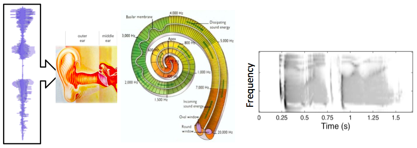
Diagram showing peripheral auditory processes. The input is shown on the left, and is processed to produce the output shown on the right.

This biological system can be modeled of as a chain of discrete sequential processes. In general, the output of each process feeds into the next process in the sequence. The model takes an array of numbers representing the acoustic waveform as its input. This is then processed by an algorithm that converts the acoustic representation to the displacement of the stapes bone within the middle ear. Following this, there is an algorithm that converts the stapes displacement into multi-channel representation of BM displacement along the cochlear partition. Next is a model of the transduction units, which convert the multichannel displacement information into a multichannel neural code representation. This is a representation of the information that would be conveyed by the auditory nerve to the brain.

The auditory model can then be used for various tasks. By making a model that can reproduce physical measurements, you can then use the model to predict the output of the system to all manner of different stimuli. For example, we know that the human auditory system is excellent at extracting speech information from noisy environments. By using the auditory model as a front end for an automatic speech recognizer, the modeler can investigate how the different components of the auditory periphery may contribute to this ability.

The basic dual resonance non-linear filterbank

There are a numerous models of cochlear mechanics. The dual resonance non-linear filterbank (DRNL) is the model developed within the Essex lab. BioAid is fundamentally a modified version of the latest version of the DRNL model.

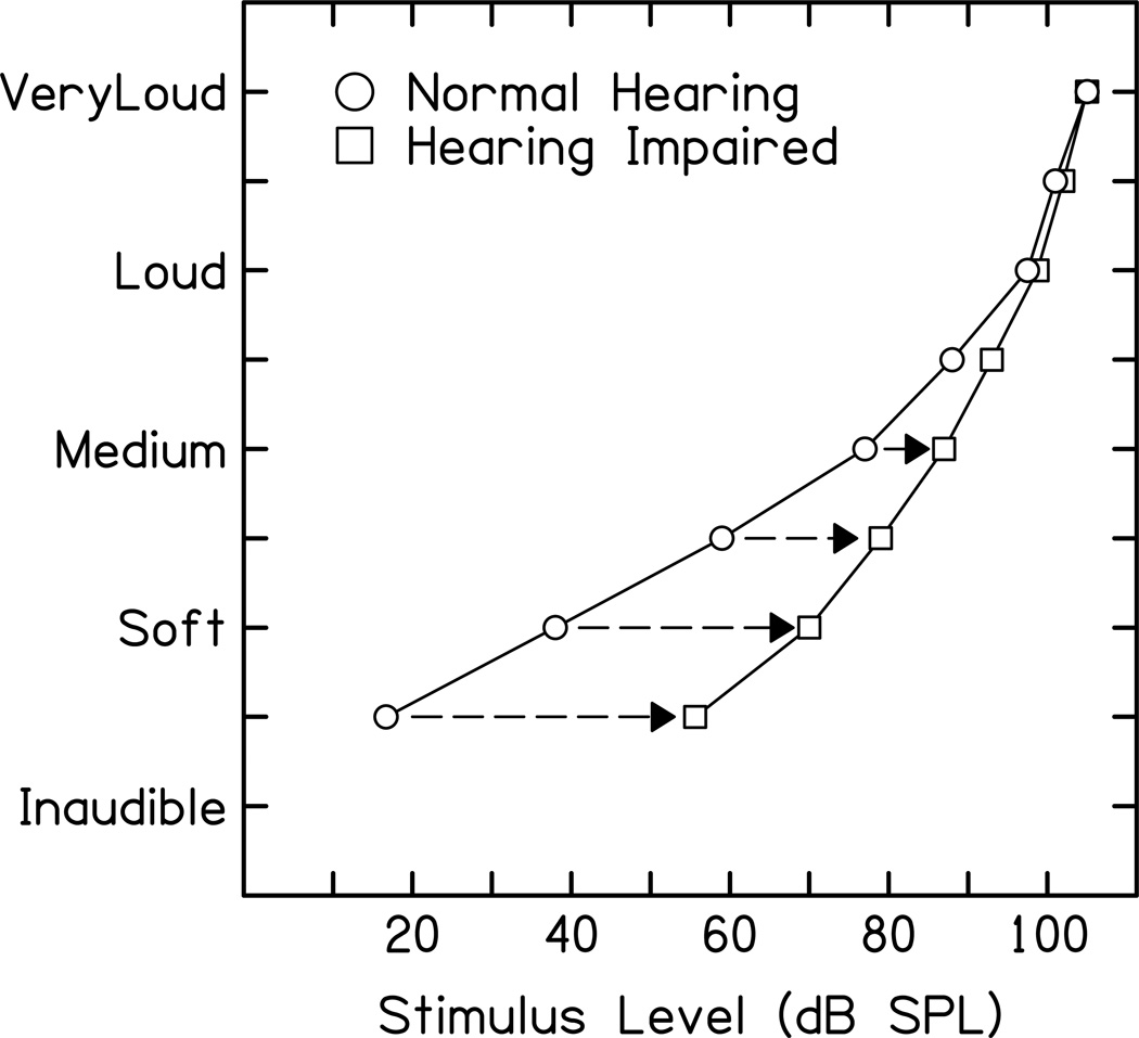
The DRNL model was originally designed to account for two major experimental observations. The first observation is the non-linear relationship of BM displacement relative to stapes displacement. This is shown by the diagram below. The basilar membrane displacement has a linear relationship with stapes displacement at low stimulus intensities. For a large part of the auditory intensity range (approximately 20 dB to 80 dB SPL across most of the audible frequency range), the relationship between stapes and BM displacement is compressive, i.e. the BM displacement only increases by 0.2 dB per dB increase in stapes displacement. At very high stimulus intensities, the relationship is linear, like at low intensities.

Stick

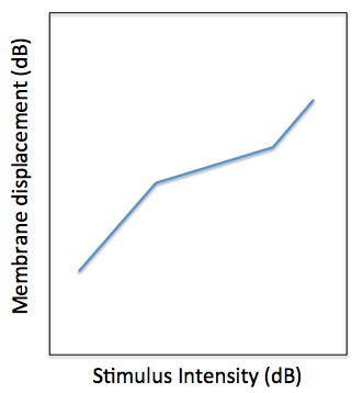
Illustration of the BM ‘Broken Stick’ non-linearity. The x-axis is the input stapes displacement and the y-axis is the output BM displacement.

The second observation is related to the relationship between the frequency selectivity of the BM with level. Each point along the BM displaces maximally at a specific frequency. Parts of the BM near to the interface with the stapes (base) respond maximally to high frequencies, while the opposite end (apex) responds maximally to low frequencies. For this reason, different regions along the basilar membrane can be thought of as filters. At low stimulus levels, the regions are highly frequency selective, so do not respond much to off-frequency stimulation. However, at higher stimulus intensities, the BM has a reduced frequency selectivity, meaning that the BM will be displaced by a proportionately greater amount when off frequency stimuli have high intensity. Not only does the bandwidth of the auditory filters change with stimulus intensity, but the centre frequency (or best frequency) also shifts.

Filter

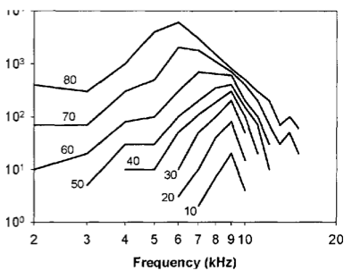
Illustration of level dependent frequency selectivity. Each line shows data from a different stimulus intensity. The x-axis is stimulus frequency and the y-axis is BM displacement for a fixed position along the membrane.

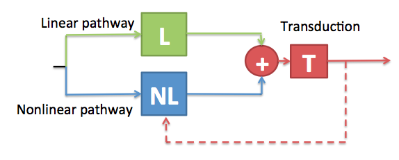
The DRNL is a parallel filterbank model, in that each cochlear channel along the BM is modeled using a an independent DRNL section. Each frequency channel of the DRNL model is comprised of two independent processing pathways. These pathways share a common input and the outputs of the pathways are summed to give the final displacement value for the location along the BM being modeled. The linear pathway is made of a linear gain function and a bandpass filter. The nonlinear pathway is made of an instantaneous broken stick non-linearity sandwiched between two bandpass filters. The filters are tuned according to the position along the BM being modeled. This arrangement is shown by the diagram below.

Filter

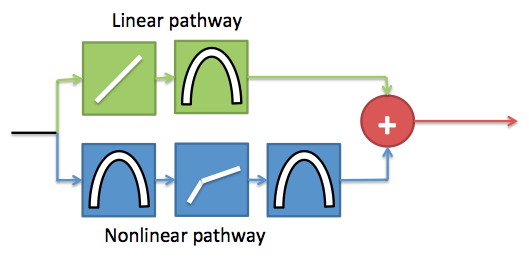
Schematic showing one frequency channel of the DRNL model

The linear pathway simulates the passive mechanical properties of the cochlear. Therefore, the output of this pathway in isolation would give the BM displacement if the active structures in the cochlear were not functioning. Conversely, the non-linear pathway is the contribution from the active mechanisms to the displacement. The 3-part piecewise relationship between BM and stapes displacement can be modeled by just summing the responses of the pathways. When performing decibel addition, the sum value is approximately the greater of the two values being summed. The output of each pathway is shown below, along with the sum total. The parameters are tuned so that the output of the model can reproduce experimental observations of BM displacement.

Filter

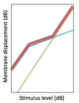
The green line is the input-output (IO) function relating stapes to BM displacement of the linear pathway of the DRNL model. The blue line is the IO function for the non-linear pathway. The red line is the decibel sum of the two pathways.

The DRNL model can also reproduce the level-dependent frequency selectivity data using this architecture. For this, the filters in the two pathways are tuned differently. As the level of stimulation increases, the contribution of the linear pathway becomes significant. By using different filter tunings, it is possible to make a level-dependent frequency response using this combination of linear filters.

The latest dual resonance non-linear filterbank

The active structures in the cochlear that give rise to the non-linear relationship between stapes- and BM-displacement are subject to control by a frequency-selective feedback pathway originating in the brain. When there is neural activity in this feedback pathway, the contribution of the active structures to BM displacement is reduced. The level of activity in the feedback network is at least partially reflexive: the feedback is activated when the acoustical stimulation intensity passes a certain threshold within a given frequency band, then grows with increasing stimulus intensity.

Robert Ferry showed that the result of neural activity in the biological feedback network could be simulated by attenuating the input to the non-linear pathway of the DRNL model. The cochlear and neural transduction processes have limited dynamic ranges, and there is some evidence to suggest that the feedback modulated attenuation may assist a listener by optimally regulating the cochlear operating point for given background noise conditions.

We subsequently went on to complete the feedback loop in the computer model. This was achieved by deriving a feedback signal from the simulated neural information to modulate the attenuation value. This complete feedback model can then adjust the attenuation parameter over time to regulate the cochlear operating point in accordance with changes in the acoustical environment. Data from automatic speech recognition experiments have shown that machine listeners equipped with the feedback network consistently outperform (i.e. correctly identify a greater proportion of the speech material) machine listeners without the feedback network in a variety of background noises.

feedback

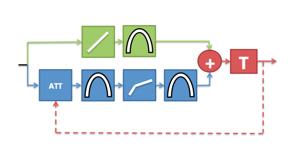
Diagram depicting the latest version of the DRNL model. The feedback signal is derived from the neural data after displacement to neural transduction stage (T). This feedback signal is used to modulate the amount of attenuation applied to the non-linear pathway over time.

Simulating hearing impairment

Some origins of hearing impairment are a result of a malfunction of certain parts of the auditory periphery. Some components of the auditory periphery are far more susceptible to failure (or reduced functionality) than others. These components can include a reduction in the function of the active structures in the cochlear that influence the BM displacement, and/or a reduction in the effectiveness of the transduction structures that convert BM displacement into neural signals.

feedback_simplified

Simplified diagram of the DRNL model to highlight the impact of reduced peripheral component functionality on cochlear feedback.

Firstly, consider the case where the transduction units within a given channel are not functioning properly. Not only is there going to be an adverse effect on the quality of the information transmitted via this channel to the brain, but the feedback loop which is driven by the neural information will also not function optimally, thus compounding the problem.

Secondly, consider the case there the active structures are not functioning correctly. This will result in a reduced BM displacement for a given level of stapes displacement. The output of the transduction units will therefore be reduced, and so the feedback will be derived from a reduced-fidelity signal. To make things worse, any residual feedback signal will not be effective because the feedback signal modulates the action of the active components, which in this case are not functioning correctly.

BioAid is designed to artificially replace the peripheral functionality that may be reduced or missing in hearing impaired listeners. By simulating the non-linear pathway and feedback loop, BioAid can at least partially restore the function of the regulating mechanisms that help normal-hearing listeners to cope when listening in noisy environments.

BioAid Architecture

algo picture

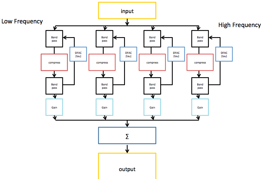
The image shows the architecture of the BioAid algorithm in block form. Only 4 channels are displayed for simplicity.

The first stage of processing in BioAid involves a decomposition of the signal into various bands. This is to coarsely simulate the frequency decomposition performed by the cochlea. The frequency decomposition performed in the BioAid app is done by a simple bank of 7 non-overlapping octave-wide Butterworth IIR filters centered at standard audiometric frequencies between 125 and 8000 Hz. When the signal is filtered twice (by first and second stage filters in the algorithm), the crossover points of each channel intersect at -6dB. This means that the energy spectrum is flat when the the channels are summed. The filters are each 2nd order. Even order filters must be used to prevent sharp phase cancellations at the filter crossover points. In the laboratory version of the aid, we have found some benefit to using an 11 channel variant of the algorithm, with additional channels between 500 and 1000, between 1000 and 2000, between 2000 and 4000, and between 4000 and 8000 Hz.

No phase correction network is used, as group delay differences between channels are not a primary issue when using wide bands with modest roll-off. For a higher frequency resolution, a filterbank with good reconstruction properties would be required. The optimum frequency resolution for this algorithm is still a research question. However, the really unique features of BioAid are related to the time domain dynamics processing that occurs within each band.

Within each band is an instantaneous compression process to simulate the action of the active components in the auditory periphery. Below the compression threshold, the input and output signals have a linear relationship. Above a certain threshold the waveform is shaped so that the only increases by 0.2 dB per dB increase in input level. In the code, this is implemented as a waveshaping algorithm that directly modifies the sample values, although it could be implemented equally effectively as a conventional side-chain compressor with zero attack and release time. Instantaneous compression is not commonly used in conventional hearing aid algorithms, as it introduces distortion. Normal hearing listeners find this distortion particularly unpleasant. However, we believe that some distortion may be useful to an impaired listener if it mimics that which occurs naturally in a healthy auditory system.

Following the instantaneous compression stage, the signal is filtered by a secondary bank of filters with the same transfer function as the first bank of filters. The instantaneous compression process introduces harmonic distortion that extends above the frequency range of the band-limited signal. It can also produce intermodulation distortion products that extend above and below the band. The secondary filter bank reduces the spread of signal energy across the frequency spectrum. Astute readers will notice that the secondary filtering means that the net compressive effect can no longer be described as instantaneous, but this is a discussion for the next blog post.

The output of the secondary filter stage is then used to generate a feedback signal. This is similar to the feedback signal implemented in the latest DRNL model, but for a reduction in computational cost, it is derived directly from the stimulus waveform (omitting models of neural transduction and low-level brain processes). We call this feedback signal the Delayed Feedback Attenuation Control (DFAC) when discussing it in the context of the hearing aid. This signal is used to modulate the level of attenuation applied to the input of each instantaneous compressor. The feedback signal has a threshold and a compression ratio like the instantaneous compressor, but it also has an integration time constant (tau) and delay parameter. Rather than modify the signal on a sample by sample basis, the DFAC integrates sample magnitude using an exponential window. This signal supplied to the integrator is delayed by 10 ms (using a ring buffer) to simulate the neuronal delay measured in the biological analogue of this process. The compression threshold value is then subtracted from the integrated value and multiplied by the compression ratio to give an attenuation value for the next sample.

The implementation of the algorithm in the app is mono. However, the algorithm code can be used in a stereo configuration (we use a stereo configuration when evaluating the algorithm in the lab). When a stereo signal is supplied, the DFAC attenuation is averaged between left and right channels. This means that the attenuation applied is identical in left and right channels within a certain frequency band. This linked setup prevents the DFAC from scrambling interaural level difference cues that might be useful to the listener. In contrast, the instantaneous compression processing is completely independent between left and right channels.

In a nutshell, each channel of BioAid is a laggy feedback compressor with an instantaneous compressor sandwiched between its attenuation and detection stages. This simple arrangement is completely unique to BioAid, and certainly quite unlike the automatic gain control circuits found in standard hearing aids.

After the secondary filtering, we depart from our adherence to physiological realism in the main signal chain. All of the processing up to this point has been focused on reducing the signal energy. To make sounds audible to hearing impaired listeners, a gain must be provided in the impaired frequency regions. This is done on a channel-by-channel basis before the signals from each of the channels are summed and then presented to the listener.

Summary

In this blog post I have described the architecture of the DRNL filterbank and how the non-linear pathway of the DRNL model forms the core of the BioAid algorithm. In the next post I will describe the unique properties of this algorithm.

BioAid Part 1: Motivations for Building a New Class of Hearing Aid

Just before Christmas, I submitted a free app (BioAid) to the Apple iTunes Store that turns an iOS device into a hearing aid. It does this by taking the audio stream from the internal microphone, processing the audio in real time, and then playing the audio back over headphones connected to the device. For more general information on usage, please visit the main BioAid site. This information is placed on my blog, allowing me to rapidly, and informally communicate some of the technical details related to the project while I gather thoughts in preparation for a more rigorous account. This is the first part of a series of posts that I intend to write about the project.

BioAid Screenshot

Screenshot of the BioAid app running on an iPhone.

BioAid is not some gimmicky sound amplifier app. The development and evaluation of the algorithm has been conducted by a team of researchers within the hearing research laboratory at the University of Essex. Our research group became involved in the development of an ‘aid on a phone’ out of necessity. BioAid is a novel design for a hearing aid that is still in its infancy. There was little chance of having it made up as a conventional hearing aid for a number of reasons. We could test it in the laboratory (using a setup described below) but convincing a manufacturer to adopt the algorithm would require a considerable financial investment. Making a case would be difficult even if our new ideas were to provide a small improvement to an established design. However, we wanted to do something much more radical. I realised that we could move directly into production using a mobile phone as a portable experimental hearing aid. This would allow us to demonstrate the viability of the concept and learn from the experiences of people all around the world, not just in our laboratory.

Laboratory tests with hearing-impaired volunteers are still in progress. These tests are being conducted using a ‘lab-scale’ version of BioAid, comprised of standard behind the ear (BTE) hearing aids that are connected to a laptop computer. The signal processing that would normally occur within the hearing aid is offloaded to the laptop, making it easier for us to change the parameters in the hearing aid at runtime, or even tweak the algorithm structure itself. Another avenue of research uses the algorithm to pre-process acoustic stimuli in an off-line mode (not real time) before they are presented to listeners over headphones. Therefore, it is important to think of BioAid as an algorithm concept, rather than to pigeon-hole it as an iOS app. The BioAid algorithm has potential for use in many applications, and the iPhone app is just one form in which BioAid exists. Another one of the numerous motivations for making the iPhone implementation was that it might inspire others to use the algorithm in unusual ways, perhaps for processing speech in a VIOP application, or as a hack for a media centre, allowing film and television audio to be processed at the source. This is why the source is freely available at GitHub. There is also a Facebook page that I encourage anyone interested in the project to ‘like’ so that they can be periodically informed of developments.

Generic hearing aid ‘gain model’

Modern hearing aids contain all manner of signal processing wizardry to assist the impaired listener in various ways. Much effort goes into developing noise-reduction technologies, and microphone array technology coupled with beam-forming algorithms to reduce off-axis sound interference. These may help to improve speech reception, or at least alleviate some of the exhaustion associated with the increased listening effort required from impaired listeners, especially when extracting information from sounds of interest in cacophonous environments. Processing often includes feedback cancellation algorithms to prevent howl associated with high gain settings in conjunction with open (non occluded) fittings. Some hearing aids even transpose information from different frequency bands to others. However, these technologies are not related to the core BioAid processing.

At the heart of any hearing aid is the ‘gain model’, and the BioAid algorithm falls into this category. The most basic goal of any hearing assistive device is to restore audibility of sounds that were previously inaudible to the hearing-impaired listener. Hearing impaired listeners have a reduced sensitivity to environmental sounds, i.e. they cannot detect the low level sounds that a normal hearing listener would be able to detect, and so it can be said that their thresholds of hearing are relatively high, or raised. To compensate for this deficit, the intensity of the stimulus must be increased, i.e. gain is provided by the hearing aid. The earliest hearing aids (the ear trumpet) just provided gain.

It is important to note that a flat loss (equal loss of sensitivity across frequency) is not often observed. More commonly, there is a distinct pattern of hearing loss, where the sensitivity is different to that of normal hearing listeners at different frequencies. For a hearing aid to work effectively across the audible spectrum, it must provide differing amounts of gain in different frequency regions. Modern hearing aids decompose sounds into separate frequency bands, perform various processing tasks, then finally recombine the signal into a waveform that can be presented to the listener via a loudspeaker. BioAid processing is no different to current hearing aids regarding this general principle.

Most hearing impaired listeners will begin to experience discomfort from loud sounds at levels not too dissimilar to those with a normal hearing sensitivity*. This means that the impaired listener has a reduced dynamic range into which the important sonic information must be squeezed. If the hearing aid applies a linear gain irrespective of the incoming sound intensity, it will help the listener detect quiet sounds, but it will also make loud sounds unbearably loud. For this reason, modern hearing aids also use compression algorithms. A lot of gain is applied to low intensity sounds to help with audibility, while considerably less gain is applied to high intensity sounds, so as not to over-amplify sounds that are already audible to the listener.

The figure below (taken from this open-access publication) is shown help illustrate the concept of reduced dynamic range. It shows categorical loudness scaling (CLS) functions for a hypothetical hearing-impaired listener and a hypothetical normal-hearing listener. A test stimulus is presented at various intensities (represented by the x-axis), and the listener is asked to categorize the loudness on a rating scale (represented by the y-axis). For sounds rated as just audible, there is a large intensity difference between the normal- and impaired-hearing listener data. However, for sounds perceived as very loud, there is little or no difference between the two listeners. The normal-hearing listener’s ratings span a range of approximately 90 dB, whereas the impaired-listener’s ratings span a relatively reduced range of approximately 50 dB.

ategorical loudness scaling

Categorical Loudness Scaling functions for hypothetical normal- and impaired-hearing listeners. Taken from here.

Unfortunately, any non-linear process (including dynamic range compression) applied to the processing chain will have side effects. In order to protect the listener from sudden loud sounds, the compression algorithm needs to respond quickly. However, standard compression algorithms with rapid temporal acuity tend to make the acoustical environment sound distinctly unnatural. The action of the compressor is clearly audible and can interfere with the important information contained in the amplitude modulations of signals such as speech. Fast compression reduces the modulation depth of amplitude modulates signals, and can therefore reduce our ability to extract information from the glimpses of signal information we might otherwise receive during the low intensity dips in modulated masking sounds. Very fast compression also changes the signal to noise ratio (SNR) of steady state signal and noise mixtures. At positive SNRs, the signal is of greater amplitude than the noise signal. If compression is so fast that it works near instantaneously, then the high level peaks of the signal will not be amplified as much as the lower level peaks in the noise signal. The noise level will increase relative to the level of the signal information reducing an otherwise advantageous SNR. The resulting negative impact on speech intelligibility is compounded by any distortion introduced by the compression process. In contrast, slowly acting compression algorithms do not impose so many negative side effects. A very slow compressor acts like a person continuously adjusting the volume control of an amplifier while watching a movie: the gain is increased for the quiet spoken passages, and then decreased in the loud action sequences. This works well for sounds with slowly changing intensity, and the sound ‘quality’ is not vastly altered. However, this is problematic if the volume is cranked up for quiet spoken passages, and there is a sudden intense event in the soundtrack that nearly deafens the audience. For this reason, both fast and slow acting compression algorithms are used in modern hearing aids to get the best possible compromise**. BioAid also utilizes fast and slow acting compression.

If BioAid is a multi-band compressor with both slow and fast acting components, then how is it different to current hearing aid gain models? On the surface, BioAid looks similar, but the architecture is certainly unique, and this gives it some unique properties.

*This is with the exception of those whose hearing is affected by a problem with the transfer of energy through the middle ear, who will generally have an increased discomfort threshold in addition to a raised detection threshold. It is also worth noting that many hearing impaired listeners have a lower discomfort threshold than that of normal hearing listeners. This condition is known as hyperacusis and is an area of active research.

**Modern digital hearing aids generally work by processing blocks (or frames) of samples. Each block of samples is processed and the output buffer is filled before the next block of samples arrives. This frame based processing is part of what gives rise to a hearing aid’s latency. This latency is generally undesirable, but while it exists, it can be used for good. It gives the compression algorithm the opportunity to ‘look ahead’ a few samples and adjust its parameters in an optimum way given the information about ‘future’ events.

Technical motivation for BioAid

BioAid is unique in that the algorithm has been designed from the ground up to mimic the processes that occur in the ear. Hearing aid technology has generally evolved to solve problems with each generation of algorithm design. This incremental approach provides an increasingly refined product. However, the problem with extended design and refine methods of development, is that the returns from each design revision generally tend to diminish. There is an asymptote. This partly explains why so much effort is now expended on the development of peripheral technologies in hearing aids, away from the core gain model. Machine hearing is a related field in which performance improvements are becoming harder to obtain using refinements of standard methods. In that field, there is a change going on, whereby radically different signal processes are being researched that are based on more physiologically accurate models of human hearing. Following in this revolutionary zeitgeist, BioAid is an effort to break through a current intellectual plateau in hearing aid gain model design.

The human auditory periphery (sound processing associated with the ear and low-level brain processing) can be modeled of as a chain of discrete sequential processes. In general the output of each process just feeds into the next process in the sequence. There are also some feedback signals that originate in processes situated further along the chain that modulate the behavior of the earlier-stage systems. The PhD thesis of Manasa Panda demonstrates that it is possible to model common hearing pathologies by reducing the functionality of, or completely removing some of the processing blocks in the chain. This modified model is called a ‘Hearing Dummy’, as the models of the periphery can be tailored to individual listeners. An artificial (machine) listener will make the same responses in hearing tests as the human when connected to their personalized Hearing Dummy.

Having isolated the components of the model likely to cause the listening difficulties, we then thought it might be a good idea to replicate those processes in a hearing aid. This could be to assist some residual functionality of certain auditory components, or to completely replace lost functionality of others. BioAid can be thought of as a simplified auditory model, containing a chain of models of the components most susceptible to the malfunctions responsible for hearing impairments.

There is one major difference between BioAid and the peripheral model used in the lab. In a standard model of the auditory periphery, the output is a code made of neural spikes representing the transformed sound information. Information in this form is useful for higher stages of brain processing with the correct interface, but it cannot be played back through a hearing aid. BioAid must deviate from the physiological model, as the sound must be recombined into a waveform that can be presented to the listener acoustically. Apart from this necessary alteration, we aim to remain faithful to the physiological model. This allows us to observe emergent properties of the system, rather than deliberately engineering properties into it.

Next Time

For those who want a technical overview of the whole project immediately, there is a YouTube video below containing a 42 minute screencast of a talk that I gave back in September 2012.

This post has described general hearing aid technology and some of scientific the motivations for developing a new class of hearing aid. In the next posts, I will discuss the algorithm structure and its properties.

Cobalt Theme for Matlab

| Comments

This is a quick post showing how to apply a cobalt-like theme to Matlab’s workspace and editor. Matlab has rather limited font and colour customization options compared to XCode (see my other post about the Cobalt theme) but it is still possible to change the default theme to something that I personally find a little easier on the eyes.

The default Matlab theme (when viewed on a Mac) is shown below …

raw

The end result is this …

cobalt

If you like the look of this, make a file called matlab.prf containing the text at the end of this post. Navigate to the folder containing the original matlab.prf, make a backup of the original file and replace it with the new version. In *nix systems, this file is located in …

1
$HOME/.matlab/<version>/matlab.prf. 	

Below is the config text …

1
2
3
4
5
6
7
8
9
10
11
12
13
14
15
16
17
#MATLAB Preferences
#Wed Jan 23 15:55:28 GMT 2013
Color_CmdWinWarnings=C-39936
Color_CmdWinErrors=C-1703936
Colors_M_UnterminatedStrings=C-5111808
Colors_M_SystemCommands=C-16022329
ColorsBackground=C-16701878
Colors_M_Warnings=C-27648
ColorsText=C-1
Colors_M_Errors=C-65536
Colors_M_Keywords=C-20124
Colors_HTML_HTMLLinks=C-16711681
Colors_M_Strings=C-16711936
ColorsUseMLintAutoFixBackground=Btrue
Colors_M_Comments=C-16711681
ColorsUseSystem=Bfalse
Desktop.Font.Code=F0 12 Monaco

Audiophile AirPlay With Raspberry Pi: Part 1

| Comments

I had recently been looking into purchasing an Apple TV for the purpose of streaming audio via AirPlay. I have little interest in the video side of things, so I started searching for a dedicated audio solution, hoping to find a high fidelity airplay receiver. Given that AirPlay data is transmitted using a lossless codec, the potential for super-high fidelity is unlimited.

After a little searching I found that a Raspberry Pi (RPi) could be converted into an airplay receiver. The only problem is the somewhat-less-than-perfect analogue audio output built into the RPi. The digital to analogue converter (DAC) in the RPi works using the pulse-width modulation (PWM) principle to keep costs down. Most high fidelity audio DACs work using the pulse-code modulation (PCM) principle, generally resulting in a more faithful representation of the digitally-encoded analogue signal.

A PWM signal is comprised of a rapid series of electrical pulses. The pulse can either be zero voltage, or maximum voltage. The width (or duty cycle) of the very rapid pulses is modulated such that the the desired output voltage is represented by the average voltage of the pulse train. This is then lowpass filtered to give a steady analogue voltage (the cutoff frequency of the filter can be well above the audible band). The pulse rate in the RPi is fixed at 100 MHz. The bit depth of this pulse stream is 1 bit (the pulse voltage can only be zero or maximum). The fixed pulse rate gives an upper limit on the amount of information that can be transmitted by the audio output built into the RPi. The following formula can be used to estimate the bit depth at the standard CD sampling rate of 44.1 kHz.

This gives us a theoretical maximum of around 11 bits / sample at 44.1 kHz. This is absolutely fine for basic speech intelligibility when running a VIOP application, or for simple sound effects. However, for any serious music listening, at least 16-bit audio is required to get full resolution dynamic range out of CDs. This means that an external USB audio interface is required, but thankfully, there are some great USB external interfaces available.

The Hardware

I happened to have a Creative X-Fi HD laying around that I was able to temporarily repurpose. This is certainly not the best external DAC that money can buy, but it sounds very good for its price, and it is more than adequate for the initial testing phase of this project.

xFi HD

The assembled test rig is shown in the screenshot below. The power is supplied by the USB hub. The xFi current draw is fairly low, meaning it can be powered from the RPi using a Y-cable if desired. The networking is wired for the time being, but the setup could easily be changed to use wifi (I have found the ALFA Networks high power USB wifi devices to work very well compared to the small Edimax devices, but this is a whole other blog post). This setup is not very visually appealing, but it is functional, and this is just the pilot phase. I have been testing this setup by streaming music from my mac using iTunes, through the test equipment, and then onwards to some Rogers LS7t speakers. I have been listening for hours on end over the past few days without noticing a single audio drop or glitch.

The sound quality is great. As far as I can tell, the digital data stream to the USB interface is uninterrupted and error free, meaning sound quality is exactly as if the Mac was directly connected to the the X-Fi Sound interface. Many people on the official Raspberry Pi forums have reported having difficulty getting stable audio when using an external USB interface. The rest of this blog article describes the software steps involved in getting pristine AirPlay audio through an external USB sound interface connected to the RPi.

Ugly, but does the job marvelously

Preparation

Before we begin, make sure that you have the Debian Wheezy operating system installed, and that you have secure shell (SSH) access to your RPi (the instructions for doing so are beyond the scope of this tutorial, but the steps required can easily be found by searching the web). Make sure that you can log onto the RPi over the network before proceeding.

The very first step is to upgrade the packages on the RPi. As root, do the following …

1
2
root@raspberrypi:~# aptitude update
root@raspberrypi:~# aptitude upgrade

On my system, the uname command gives the following output (so long as the output you see has the same date stamp, or is newer, then things should be OK) …

1
2
pi@raspberrypi ~ $ uname -a
Linux raspberrypi 3.6.11+ #348 PREEMPT Tue Jan 1 16:33:22 GMT 2013 armv6l GNU/Linux

The next step is to upgrade the RPi’s firmware. As root, use the following command …

1
root@raspberrypi:~# rpi-update

For me, this failed on the first run, but worked OK on the second attempt. For detailed information regarding the rpi-update command, see the associated github repository.

Test AirPlay using the onboard sound

This section is a summary of the instructions found here. The default audio output should be set to the onboard stereo jack. For this, a single command is required as root …

1
root@raspberrypi:~# amixer cset numid=3 1

Before download and compilation of the shairport software (this is the software that makes the RPi mimic an authentic AirPlay device), some prerequisites need to be installed. As root, install the following packages …

1
root@raspberrypi:~# aptitude install git libao-dev libssl-dev libcrypt-openssl-rsa-perl libio-socket-inet6-perl libwww-perl avahi-utils

I also needed to get the Net::SDP perl library when I tried this. This was done using the following command as root …

1
root@raspberrypi:~# cpan install Net::SDP

With all the prerequisites successfully installed, the next step is to download shairport sources and compile them as root …

1
2
3
root@raspberrypi:~# git clone https://github.com/albertz/shairport.git shairport
root@raspberrypi:~# cd shairport
root@raspberrypi:~/shairport# make

Shairport can now be tested by launching it in the foreground …

1
root@raspberrypi:~/shairport# ./shairport.pl -a AirPi

… and then connecting to it using an AirPlay compatible device. The streamed data should then be audible from the 3.5 mm jack with speakers or headphones attached.

Getting an external USB DAC to work without pops / clicks / noise

Firstly, install some prerequisites as root …

1
2
3
root@raspberrypi:~# apt-get install libasound2-plugins
root@raspberrypi:~# apt-get install libesd0
root@raspberrypi:~# apt-get install nas

The next step is to edit /boot/cmdline.txt to fix some of the potential causes of pops when using a USB sound interface. Open /boot/cmdline.txt in the nano editor as root …

1
root@raspberrypi:~# nano /boot/cmdline.txt

Add the following text to the file. I’m not sure if the position of the text makes a difference, but I appended the text to the front of the existing text. Once the text has been added, quit the nano editor using ctrl+x and save the changes by hitting return when prompted.

1
dwc_otg.speed=1 dwc_otg.fiq_fix_enable=1 

Using nano as in the previous step (or your favorite editor), edit /etc/libao.conf so that it contains the following …

1
2
3
default_driver=alsa
dev=default
use_mmap=no

Edit /etc/modprobe.d/alsa-base.conf, commenting out the snd-usb-audio line and adding the snd_bcm2835 line so part of the file looks like the following …

1
2
#options snd-usb-audio index=-2
options snd_bcm2835 index=-2

For testing purposes, create a hidden file, .asoundrc, in the home directory of a regular user. For example, as pi …

1
pi@raspberrypi ~ $ touch .asoundrc

Then edit this file to contain the following configuration data…

1
2
3
4
5
6
7
8
9
10
11
12
13
14
15
16
17
18
19
20
21
22
23
24
25
26
27
28
29
30
31
32
33
34
35
36
37
38
39
40
41
42
43
44
45
46
47
48
49
50
51
52
53
54
55
pcm.!default {
    type plug
    slave.pcm "softvol"
}
pcm.dmixer {
       type dmix
       ipc_key 1024
       slave {
           pcm "hw:0"
           period_time 0
           period_size 4096
           buffer_size 131072
           rate 44100
       }
       bindings {
           0 0
           1 1
       }
}
pcm.dsnooper {
       type dsnoop
       ipc_key 1024
       slave {
           pcm "hw:0"
           channels 2
           period_time 0
           period_size 4096
           buffer_size 131072
           rate 1
       }
       bindings {
           0 0
           1 1
       }
}
pcm.softvol {
       type softvol
       slave { pcm "dmixer" }
       control {
           name "Master"
           card 0
       }
}
ctl.!default {
    type hw
    card 0
}
ctl.softvol {
    type hw
    card 0
}
ctl.dmixer {
    type hw
    card 0
}

Restart the RPi before proceeding. Attach the external USB sound interface to some speakers or headphones, manually start up shairport again like in the previous example, then test it by connecting to the shairport server and streaming some music

1
root@raspberrypi:~/shairport# ./shairport.pl -a AirPi

If this all works OK, then make a demon process so that shairport always runs on startup or after the RPi is reset.

Running the AirPort server at startup

The first task is to copy the local .asoundrc to /etc/asound.conf so that it can be found by the demon process. This tripped me up for a bit!

1
root@raspberrypi:~# cp /home/pi/.asoundrc /etc/asound.conf

As root, install the shairport software, copy the default configuration, make the shairport init script executable, and then update rc.d by issuing the following commands …

1
2
3
4
5
root@raspberrypi:~/shairport# make install
root@raspberrypi:~/shairport# cp shairport.init.sample /etc/init.d/shairport
root@raspberrypi:~/shairport# cd /etc/init.d
root@raspberrypi:/etc/init.d# chmod a+x shairport
root@raspberrypi:/etc/init.d# update-rc.d shairport defaults

Before starting the daemon, we have to add the AP Name in the launch parameters. Edit the file using nano shairport then change the DAEMON_ARGS variable line so it looks like the following …

1
DAEMON_ARGS="-w $PIDFILE -a AirPi"

Replace AirPi with whatever you want it to appear as on your network. The demon can be started using the following …

1
root@raspberrypi:/etc/init.d# ./shairport start

The AirPlay service will now start whenever the RPi is powered on.

Coming soon

In the next installment of this blog series, I will attempt to interface the Raspberry Pi with a Schiit Modi dedicated USB DAC. I have one on order from the manufacturer in the USA (it is currently in the post). These are supposed to provide incredible sound quality for the price. the problem with the xFi is that it tires to do too much (optical / audio in / headphone amp). the Modi just has a USB input and a stereo line level analogue output. As an AipPlay device for use with the Raspberry Pi, no money (or size) is wasted on superfluous functionality.

In the next installment, I also intend to some controlled tests to compare the setup’s sound quality to an Apple TV. I’ll do this with a number of listeners. I’m excited to find out what happens!

UPDATE: Seeing as this post generates the most traffic on my blog, I’d like to add a shameless plug www.aud1.com to my latest project.

Cobalt Theme for Xcode

| Comments

I am very fond of the TextMate 2 open source editor. I use it to write posts for this blog. I also really like the ‘cobalt’ text formatting theme that is included with TextMate.

I do not like the hideous default themes that ship with Xcode, and neither does this guy. Daniel Barowy kindly supplies a cobalt emulation theme for xcode on his site, but the file format does not work with the latest version of XCode. I converted this theme and tweaked it slightly to darken the appearance console output. The screenshot below shows Xcode adjacent to TextMate.

If you like the look of this, then copy and paste the text from the code box below into the following file.

1
~/Library/Developer/Xcode/UserData/FontAndColorThemes/cobalt.dvtcolortheme

Finally, restart Xcode and select the Cobalt theme under the preferences menu.

cobalt.dvtcolortheme
1
2
3
4
5
6
7
8
9
10
11
12
13
14
15
16
17
18
19
20
21
22
23
24
25
26
27
28
29
30
31
32
33
34
35
36
37
38
39
40
41
42
43
44
45
46
47
48
49
50
51
52
53
54
55
56
57
58
59
60
61
62
63
64
65
66
67
68
69
70
71
72
73
74
75
76
77
78
79
80
81
82
83
84
85
86
87
88
89
90
91
92
93
94
95
96
97
98
99
100
101
102
103
104
105
106
107
108
109
110
111
112
113
114
115
116
117
118
119
120
121
122
123
124
125
126
127
128
129
130
131
132
133
134
135
136
137
138
139
140
141
142
<?xml version="1.0" encoding="UTF-8"?>
<!DOCTYPE plist PUBLIC "-//Apple//DTD PLIST 1.0//EN" "http://www.apple.com/DTDs/PropertyList-1.0.dtd">
<plist version="1.0">
<dict>
	<key>DVTConsoleDebuggerInputTextColor</key>
	<string>0.908811 0.908811 0.908811 1</string>
	<key>DVTConsoleDebuggerInputTextFont</key>
	<string>Menlo-Bold - 11.0</string>
	<key>DVTConsoleDebuggerOutputTextColor</key>
	<string>0.851394 0.851394 0.851394 1</string>
	<key>DVTConsoleDebuggerOutputTextFont</key>
	<string>Menlo-Regular - 11.0</string>
	<key>DVTConsoleDebuggerPromptTextColor</key>
	<string>0.38565 0.777779 1 1</string>
	<key>DVTConsoleDebuggerPromptTextFont</key>
	<string>Menlo-Bold - 11.0</string>
	<key>DVTConsoleExectuableInputTextColor</key>
	<string>0.971012 0.971012 0.971012 1</string>
	<key>DVTConsoleExectuableInputTextFont</key>
	<string>Menlo-Regular - 11.0</string>
	<key>DVTConsoleExectuableOutputTextColor</key>
	<string>0.971012 0.971012 0.971012 1</string>
	<key>DVTConsoleExectuableOutputTextFont</key>
	<string>Menlo-Bold - 11.0</string>
	<key>DVTConsoleTextBackgroundColor</key>
	<string>0 0 0 1</string>
	<key>DVTConsoleTextInsertionPointColor</key>
	<string>0 0 0 1</string>
	<key>DVTConsoleTextSelectionColor</key>
	<string>0.576266 0.81005 1 1</string>
	<key>DVTDebuggerInstructionPointerColor</key>
	<string>0.705792 0.8 0.544 1</string>
	<key>DVTSourceTextBackground</key>
	<string>0 0.133 0.251 1</string>
	<key>DVTSourceTextBlockDimBackgroundColor</key>
	<string>0.5 0.5 0.5 1</string>
	<key>DVTSourceTextInsertionPointColor</key>
	<string>1 1 1 1</string>
	<key>DVTSourceTextInvisiblesColor</key>
	<string>0.5 0.5 0.5 1</string>
	<key>DVTSourceTextSelectionColor</key>
	<string>0.702 0.396 0.224 1</string>
	<key>DVTSourceTextSyntaxColors</key>
	<dict>
		<key>xcode.syntax.attribute</key>
		<string>0.537 0.588 0.659 1</string>
		<key>xcode.syntax.character</key>
		<string>1 0.384 0.549 1</string>
		<key>xcode.syntax.comment</key>
		<string>0 0.533 1 1</string>
		<key>xcode.syntax.comment.doc</key>
		<string>0 0.533 1 1</string>
		<key>xcode.syntax.comment.doc.keyword</key>
		<string>0 0.533 1 1</string>
		<key>xcode.syntax.identifier.class</key>
		<string>0.261 0.626 0.982 1</string>
		<key>xcode.syntax.identifier.class.system</key>
		<string>1 0.867 0 1</string>
		<key>xcode.syntax.identifier.constant</key>
		<string>0.261 0.626 0.982 1</string>
		<key>xcode.syntax.identifier.constant.system</key>
		<string>1 0.384 0.549 1</string>
		<key>xcode.syntax.identifier.function</key>
		<string>0.261 0.626 0.982 1</string>
		<key>xcode.syntax.identifier.function.system</key>
		<string>1 0.867 0 1</string>
		<key>xcode.syntax.identifier.macro</key>
		<string>0.537 0.588 0.659 1</string>
		<key>xcode.syntax.identifier.macro.system</key>
		<string>1 0.616 0 1</string>
		<key>xcode.syntax.identifier.type</key>
		<string>0.261 0.626 0.982 1</string>
		<key>xcode.syntax.identifier.type.system</key>
		<string>0.502 1 0.51 1</string>
		<key>xcode.syntax.identifier.variable</key>
		<string>0.261 0.626 0.982 1</string>
		<key>xcode.syntax.identifier.variable.system</key>
		<string>0.8 0.8 0.8 1</string>
		<key>xcode.syntax.keyword</key>
		<string>1 0.616 0 1</string>
		<key>xcode.syntax.number</key>
		<string>1 0.384 0.549 1</string>
		<key>xcode.syntax.plain</key>
		<string>1 1 1 1</string>
		<key>xcode.syntax.preprocessor</key>
		<string>0.665 0.992 0.997 1</string>
		<key>xcode.syntax.string</key>
		<string>0.227 0.851 0 1</string>
		<key>xcode.syntax.url</key>
		<string>0.227 0.851 0 1</string>
	</dict>
	<key>DVTSourceTextSyntaxFonts</key>
	<dict>
		<key>xcode.syntax.attribute</key>
		<string>Monaco - 12.0</string>
		<key>xcode.syntax.character</key>
		<string>Monaco - 12.0</string>
		<key>xcode.syntax.comment</key>
		<string>Menlo-Italic - 12.0</string>
		<key>xcode.syntax.comment.doc</key>
		<string>Menlo-Italic - 12.0</string>
		<key>xcode.syntax.comment.doc.keyword</key>
		<string>Menlo-Italic - 12.0</string>
		<key>xcode.syntax.identifier.class</key>
		<string>Monaco - 12.0</string>
		<key>xcode.syntax.identifier.class.system</key>
		<string>Monaco - 12.0</string>
		<key>xcode.syntax.identifier.constant</key>
		<string>Monaco - 12.0</string>
		<key>xcode.syntax.identifier.constant.system</key>
		<string>Monaco - 12.0</string>
		<key>xcode.syntax.identifier.function</key>
		<string>Monaco - 12.0</string>
		<key>xcode.syntax.identifier.function.system</key>
		<string>Monaco - 12.0</string>
		<key>xcode.syntax.identifier.macro</key>
		<string>Monaco - 12.0</string>
		<key>xcode.syntax.identifier.macro.system</key>
		<string>Monaco - 12.0</string>
		<key>xcode.syntax.identifier.type</key>
		<string>Monaco - 12.0</string>
		<key>xcode.syntax.identifier.type.system</key>
		<string>Monaco - 12.0</string>
		<key>xcode.syntax.identifier.variable</key>
		<string>Monaco - 12.0</string>
		<key>xcode.syntax.identifier.variable.system</key>
		<string>Monaco - 12.0</string>
		<key>xcode.syntax.keyword</key>
		<string>Monaco - 12.0</string>
		<key>xcode.syntax.number</key>
		<string>Monaco - 12.0</string>
		<key>xcode.syntax.plain</key>
		<string>Monaco - 12.0</string>
		<key>xcode.syntax.preprocessor</key>
		<string>Monaco - 12.0</string>
		<key>xcode.syntax.string</key>
		<string>Monaco - 12.0</string>
		<key>xcode.syntax.url</key>
		<string>Monaco - 12.0</string>
	</dict>
</dict>
</plist>